BEFORE
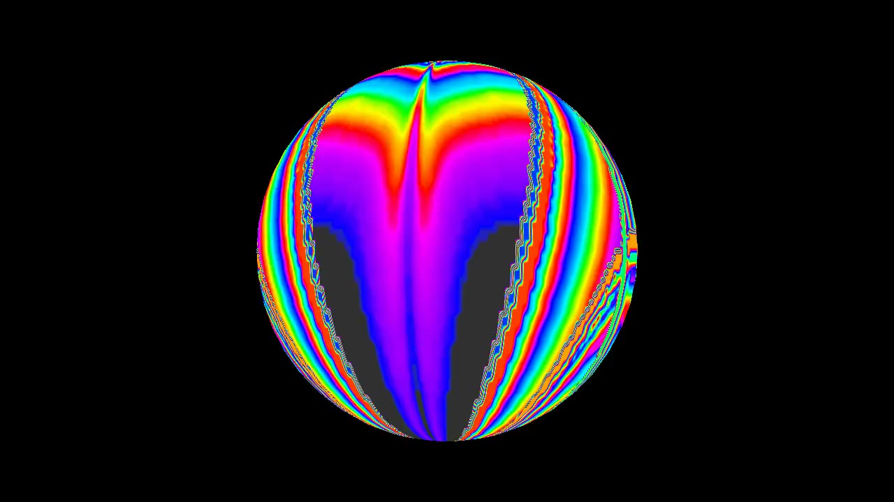
AFTER
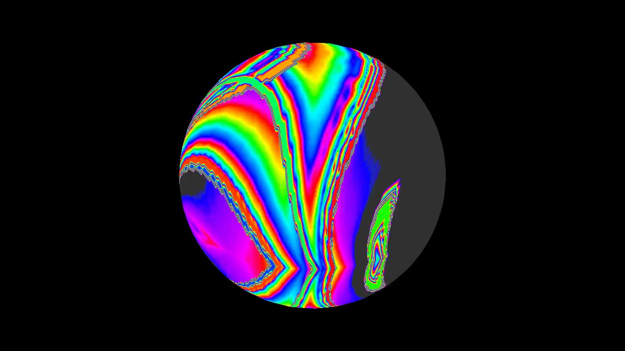
This is the third stop on our tour of curved-surface rendering artifacts, after the missing depth buffer and the wrap seam. With those two fixed, the sphere mode had one glitch left, and it lived at the poles: a pinwheel of compressed color bands converging on a single point, shimmering with moiré as the camera moved. Unlike the depth bug (a pipeline mistake) and the seam (a mathematical inevitability we softened), the pinch is a projection choice — and cartographers worked out the better choice more than four centuries ago.
ShoggothOx wraps its live 160×100 simulation buffer around the
sphere with plain latitude–longitude UV mapping: u is
longitude, v is latitude. Every horizontal row of the texture
becomes a latitude ring around the sphere (a horizontal circle parallel to
the equator, not a pole-to-pole band) — the equator gets a big ring,
and rings near the poles get smaller and smaller until, at the pole
itself, an entire row of 160 texels is crushed into a single point.
The texture content doesn't know that. Its columns keep varying all the way up, so near the pole you get 160 columns' worth of horizontal detail packed into a circle a few pixels across: a starburst of radial spokes, aliasing into moiré when it moves. Map readers know this defect from the other direction — on an equirectangular map of Earth, Antarctica smears into a continent-wide ribbon along the bottom edge. We're doing the inverse: instead of stretching the globe onto a rectangle, we're squeezing a rectangle onto a globe, so the smear becomes a pinch.
Let's put numbers on it. At colatitude φ (angle from the
pole), a latitude ring has circumference
2πr sin φ, but the old mapping assigns
every ring the same span of texture columns. The horizontal texel
density on the surface therefore grows like
1 / sin φ — and diverges at the
poles. No amount of mesh tessellation or filtering fixes that; the mapping
itself demands infinite spatial sampling frequency at two points.
The cure is to stop giving every ring the full texture width. Scale the
u span of each ring by the ring's own radius factor,
sin φ, and the divergence cancels exactly: texel
density becomes constant per unit of arc, at every latitude.
Cartographers call this the
sinusoidal projection (also Sanson–Flamsteed, in use since the
1570s).
In cartography, a sinusoidal map draws the 3D globe onto a 2D page within
a lens-shaped outline. In 3D GPU rendering, we apply this mapping in
reverse: the 3D sphere mesh queries UV coordinates from our flat 2D
rectangular simulation buffer. Because each latitude ring's UV span scales
with sin φ, the sphere surface queries a
lens-shaped footprint out of the 2D rectangular buffer.
Crucially, 100% of the 3D sphere is fully textured
— no physical gaps exist on the sphere. Because a high-latitude ring
has a smaller physical circumference in 3D space, sampling a shorter UV
interval
[1 − sin φ,
        1 + sin φ]
still covers the full 360° circumference of that ring
at the exact same spatial texel density as the equator. The 4 outer corner
regions of the 2D rectangular simulation buffer simply remain unread by
the 3D sphere mesh.
It is an equal-area projection: the Jacobian determinant of our texture-to-sphere map works out to a constant, so a blob in the simulation buffer covers the same amount of sphere surface whether it lands at the equator or near a pole.
sin φ, which
covers 100% of that ring's 360° sphere circumference at uniform
texel density. The 3D sphere surface is completely textured; only the 4
outer corner regions of the 2D rectangular texture buffer remain unread.
The implementation is a one-line change per mesh (our generating functions
for our 3d surfaces: spheres, cones, etc.), but the line has to respect
the seam fix we already
shipped. Closed directions — periodic mesh axes where
traveling continuously loops back onto itself, such as traveling 360°
around a longitude circle — traverse the mirrored coordinate span
u ∈ [0, 2]. The seam wrap is invisible
because MirrorRepeat renders the texture symmetric about the
central mirror axis u = 1. So when we shrink a
latitude ring's UV span near the poles, we must shrink it symmetrically toward the mirror center:
// crates/render/src/mesh.rs, make_sphere()
verts.push(Vertex {
    pos: [sin_p * cos_t * 0.9, cos_p * 0.9, sin_p * sin_t * 0.9],
    uv: [1.0 + (uu * 2.0 - 1.0) * sin_p, vv],   // was [uu * 2.0, vv]
});
Why the center and not, say, the left edge? Seam continuity. The two ends
of a 360° mesh loop (the longitude parameters
uu = 0 and uu = 1) land on
the exact same physical line on the sphere, so they must sample the same
texel. (Note the distinction:
uu = 0 ≡ 1 corresponds to 0°
≡ 360° at the seam line, whereas uu = 0.5
corresponds to 180° on the opposite side of the sphere where texture
coordinate u = 1 sits at the mirror fold). With the
span [1 − s, 1 + s] centered on the
fold, the mirror function sends both ends to the same place:
mirror(1−s) = mirror(1+s) =
        1−s
. The reflection symmetry that killed the seam is
exactly the symmetry that lets us shrink the span freely — the two
fixes compose instead of fighting. Three properties fall out:
sin φ = 1) the
span is [0, 2] — identical to the old mapping.
Nothing changes where the old mapping was already good.
sin φ = 0) every
vertex samples u = 1: one texel column, one well-defined
color. The pinwheel is gone by construction
— there is no varying content left to pinch.
The double cones got the same one-liner — a cone's apex is the same
degeneracy as a sphere's pole, with 1 − t
playing the role of sin φ:
// make_cones(): apex pinch, same cure
// Previous UV: [uu * 2.0, tt]
uv: [1.0 + (uu * 2.0 - 1.0) * (1.0 - tt), tt],
The torus needs nothing: it has no degenerate rings (every point of a torus looks locally like every other), which is why it never showed the artifact. And because the whole fix lives in the vertex UVs, the shader, samplers, and simulation are untouched — the GPU interpolates the new coordinates exactly as it did the old ones.
Equal-area projections pay for their honesty somewhere, and ours pays in
coverage. The lens-shaped footprint in the diagram covers
4/π of the mirrored span — about 64% — so
roughly a third of the buffer (the regions near the seam edges at high
latitudes; the "corners" of the map) is never sampled by the sphere at
all.
Does skipping the four corners of the 2D texture buffer introduce a
discontinuity or tear on the 3D sphere? No — the surface
remains perfectly smooth and continuous everywhere. In
graphics, a visual discontinuity occurs when adjacent points on a surface
jump across non-adjacent texture coordinates. Here, vertex UVs are
governed by smooth, continuous mathematical functions:
u(φ, θ) = 1.0 + (uu · 2.0 − 1.0)
        · sin φ
across the entire mesh. As latitude
moves continuously from equator to pole, the sampled UV interval narrows
seamlessly toward the center line u = 1.
Neighboring vertices on the 3D sphere always sample neighboring texels in
the 2D buffer. The corner texels in memory simply lie outside the domain
of this continuous mapping — unread locations that no vertex on the
3D sphere ever queries.
There's also shear: while lines of latitude remain horizontal circles
parallel to the equator, each ring's UV width scales with
sin φ. Away from the central meridian, vertical
lines of longitude (meridians) and vertical features in the buffer shear
and lean into sweeping curves as they climb toward the poles — the
same italic tilt you see in continents at the edge of a sinusoidal world
map. That shear is visible well away from the poles, so the sphere's whole
character shifts: where the old mapping showed rigid vertical stripes at
every latitude, the new one bends them into graceful curves as they
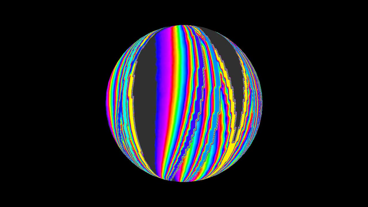
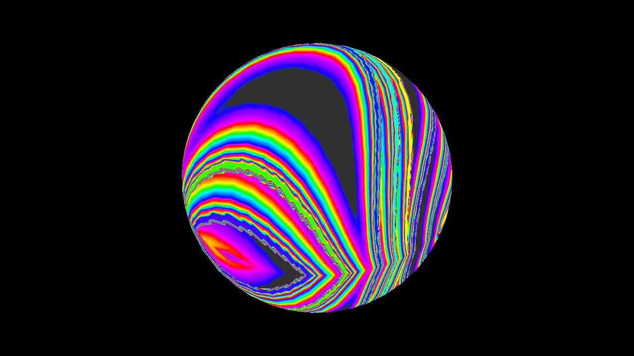
converge. Compare the before/after pairs above — it's a genuinely
different (we'd say better) look, not just a patched pole.
For a music visualizer, both are cheap. The buffer's content is a boiling, palette-cycled simulation with no privileged corner worth preserving, and the previous alternative was not "show the corners" but "shred them into a moiré pinwheel." As with the mirror symmetry, what remains reads as intentional: the bands now taper gracefully into the pole the way segments taper on a beach ball — a shape the eye already trusts.
Same protocol as the previous two fixes, thanks to the deterministic
render pipeline: re-render the reference track with the effect playlist
held fixed (cargo xtask video "8bit Dungeon Boss"
--reuse-playlist), then extract the same timestamps from both
videos. The simulation content matches frame for frame — the only
thing that changed is where each texel lands on the sphere. The
before/after pairs in this post are those frames.
That leaves two small items on the curvature-rendering list: a one-texel out-of-bounds fetch at the far edge of the height-field mesh, and a palette lookup that should use nearest-neighbor filtering instead of blending unrelated palette entries. Both get the same treatment: fix, re-render, compare.